Submarine Cable Simulation: Magnetic Fields, Losses and Heating
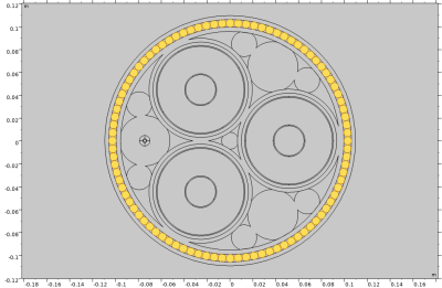
Submarine cables carry high electrical currents over long distances, generating both magnetic fields and heat within the cable system. COMSOL Multiphysics can model the magnetic fields around the cables, calculate the electromagnetic losses and determine the resulting temperature distribution and thermal behavior.
Current density and skin effect in submarine cables
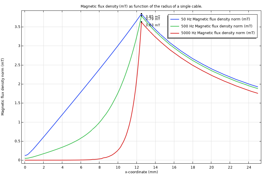
The skin effect should be taken into account in a submarine cable, especially when Joule heating is part of the analysis. The skin effect depends on the frequency of the current. At 50 Hz it is not strong, but the simulation captures it accurately. The graph shows the magnetic flux density as a function of radius. The blue line is the 50 Hz case, and the green and red lines are the 500 Hz and 5000 Hz cases.
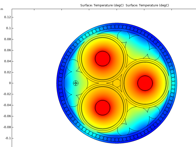
The temperature of a submarine cable must stay below a maximum value. In this example the limit is 80 °C, the copper cable carries 240 A, and the three phases are 120 degrees apart. Joule heating from the cable resistance causes the temperature rise. The thermal properties of all materials around the cable must be included to obtain a good estimate of the maximum temperature inside the cable.
Magnetic field strength in and around the cable
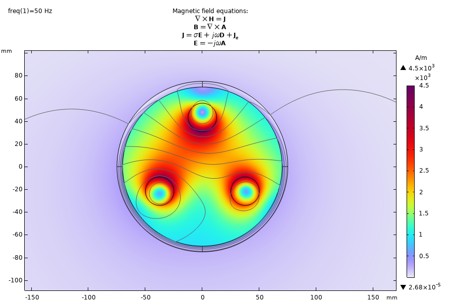
The figure shows the magnetic field strength, including the shielding effect of the steel sheath. The simulation solves Maxwell’s equations for the cable geometry. Because of the relative permeability of the steel, the magnetic field outside the cable is reduced significantly. The figure shows the 50 Hz situation.